Upmc Td Fascicule Corrige Solution Systeme Procedes Pdf
1. Reinforcement Learning 101
Typically, a RL setup is composed of two components, an agent and an environment.
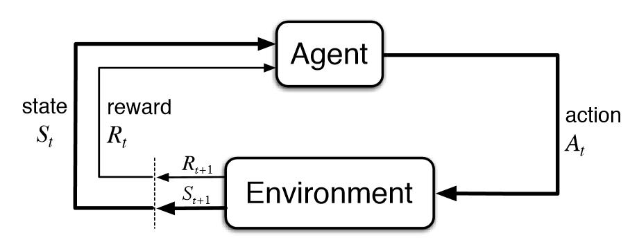
Then environment refers to the object that the agent is acting on (e.g. the game itself in the Atari game), while the agent represents the RL algorithm. The environment starts by sending a state to the agent, which then based on its knowledge to take an action in response to that state. After that, the environment send a pair of next state and reward back to the agent. The agent will update its knowledge with the reward returned by the environment to evaluate its last action. The loop keeps going on until the environment sends a terminal state, which ends to episode.
Most of the RL algorithms follow this pattern. In the following paragraphs, I will briefly talk about some terms used in RL to facilitate our discussion in the next section.
Definition
- Action (A): All the possible moves that the agent can take
- State (S): Current situation returned by the environment.
- Reward (R): An immediate return send back from the environment to evaluate the last action.
- Policy (π): The strategy that the agent employs to determine next action based on the current state.
- Value (V): The expected long-term return with discount, as opposed to the short-term reward R. Vπ(s) is defined as the expected long-term return of the current state sunder policy π.
- Q-value or action-value (Q): Q-value is similar to Value, except that it takes an extra parameter, the current action a. Qπ(s, a) refers to the long-term return of the current state s, taking action a under policy π.
Model-free v.s. Model-based
The model stands for the simulation of the dynamics of the environment. That is, the model learns the transition probability T(s1|(s0, a)) from the pair of current state s0 and action a to the next state s1. If the transition probability is successfully learned, the agent will know how likely to enter a specific state given current state and action. However, model-based algorithms become impractical as the state space and action space grows (S * S * A, for a tabular setup).
On the other hand, model-free algorithms rely on trial-and-error to update its knowledge. As a result, it does not require space to store all the combination of states and actions. All the algorithms discussed in the next section fall into this category.
On-policy v.s. Off-policy
An on-policy agent learns the value based on its current action a derived from the current policy, whereas its off-policy counter part learns it based on the action a* obtained from another policy. In Q-learning, such policy is the greedy policy. (We will talk more on that in Q-learning and SARSA)
2. Illustration of Various Algorithms
2.1 Q-Learning
Q-Learning is an off-policy, model-free RL algorithm based on the well-known Bellman Equation:

E in the above equation refers to the expectation, while ƛ refers to the discount factor. We can re-write it in the form of Q-value:

The optimal Q-value, denoted as Q* can be expressed as:

The goal is to maximize the Q-value. Before diving into the method to optimize Q-value, I would like to discuss two value update methods that are closely related to Q-learning.
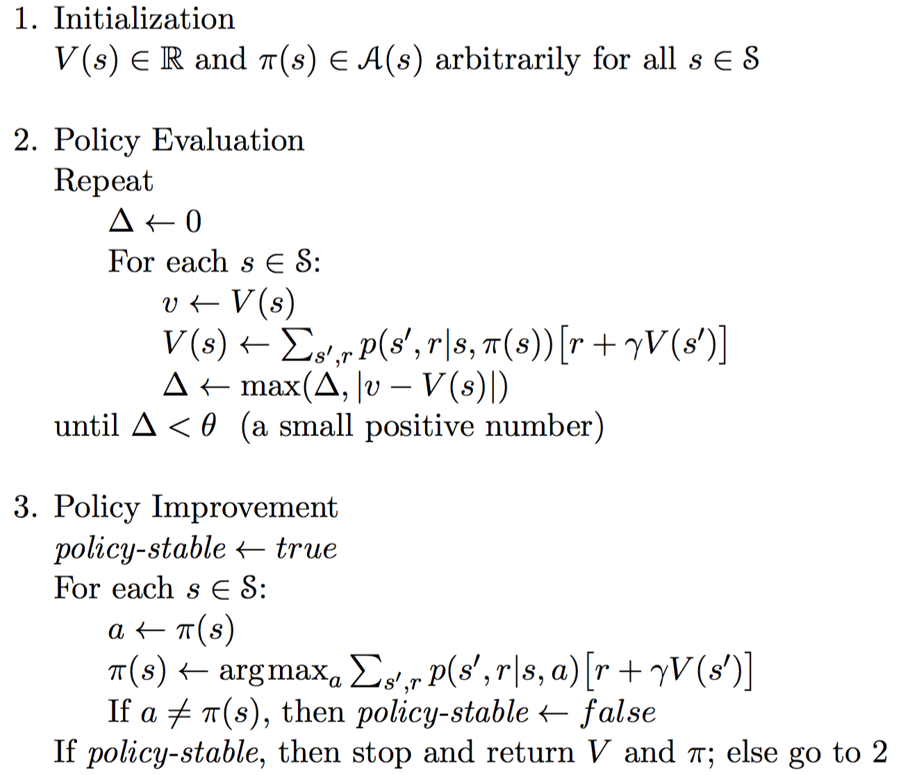
Policy Iteration
Policy iteration runs an loop between policy evaluation and policy improvement.
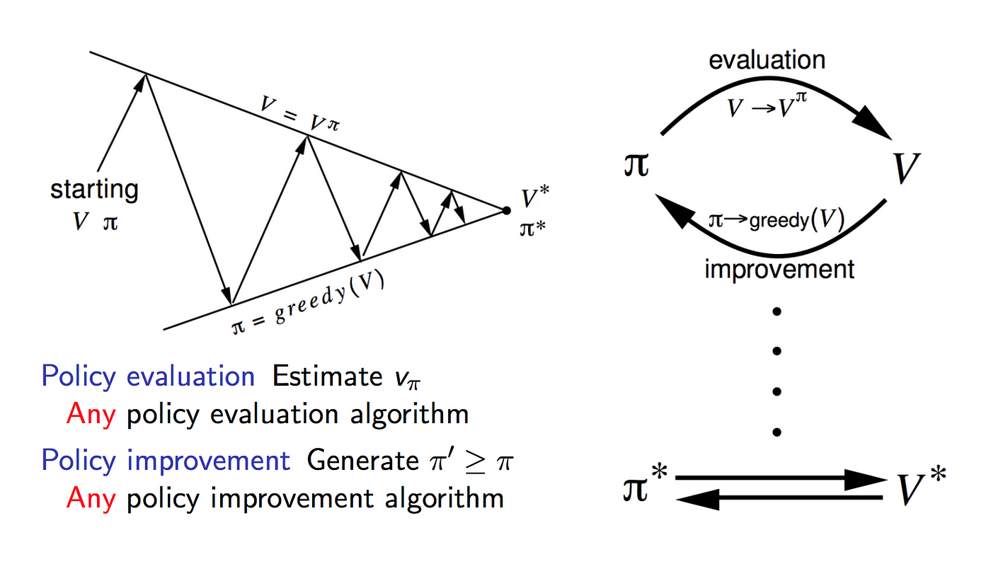
Policy evaluation estimates the value function V with the greedy policy obtained from the last policy improvement. Policy improvement, on the other hand, updates the policy with the action that maximizes V for each of the state. The update equations are based on Bellman Equation. It keeps iterating till convergence.
Value Iteration
Value Iteration only contains one component. It updates the value function V based on the Optimal Bellman Equation.
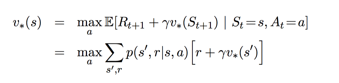
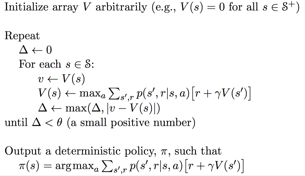
After the iteration converges, the optimal policy is straight-forwardly derived by applying an argument-max function for all of the states.
Note that these two methods require the knowledge of the transition probability p, indicating that it is a model-based algorithm. However, as I mentioned earlier, model-based algorithm suffers from scalability problem. So how does Q-learning solves this problem?

α refers to the learning rate (i.e. how fast are we approaching the goal). The idea behind Q-learning is highly relied on value iteration. However, the update equation is replaced with the above formula. As a result, we do not need to worry about the transition probability anymore.

Note that the next action a' is chosen to maximize the next state's Q-value instead of following the current policy. As a result, Q-learning belongs to the off-policy category.
2.2 State-Action-Reward-State-Action (SARSA)
SARSA very much resembles Q-learning. The key difference between SARSA and Q-learning is that SARSA is an on-policy algorithm. It implies that SARSA learns the Q-value based on the action performed by the current policy instead of the greedy policy.

The action a_(t+1) is the action performed in the next state s_(t+1) under current policy.

From the pseudo code above you may notice two action selection are performed, which always follows the current policy. By contrast, Q-learning has no constraint over the next action, as long as it maximizes the Q-value for the next state. Therefore, SARSA is an on-policy algorithm.
2.3 Deep Q Network (DQN)
Although Q-learning is a very powerful algorithm, its main weakness is lack of generality. If you view Q-learning as updating numbers in a two-dimensional array (Action Space * State Space), it, in fact, resembles dynamic programming. This indicates that for states that the Q-learning agent has not seen before, it has no clue which action to take. In other words, Q-learning agent does not have the ability to estimate value for unseen states. To deal with this problem, DQN get rid of the two-dimensional array by introducing Neural Network.
DQN leverages a Neural Network to estimate the Q-value function. The input for the network is the current, while the output is the corresponding Q-value for each of the action.
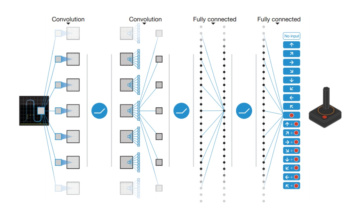
In 2013, DeepMind applied DQN to Atari game, as illustrated in the above figure. The input is the raw image of the current game situation. It went through several layers including convolutional layer as well as fully connected layer. The output is the Q-value for each of the actions that the agent can take.
The question boils down to: How do we train the network?
The answer is that we train the network based on the Q-learning update equation. Recall that the target Q-value for Q-learning is:
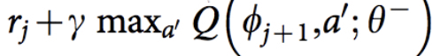
The ϕ is equivalent to the state s, while the 𝜽 stands for the parameters in the Neural Network, which is not in the domain of our discussion. Thus, the loss function for the network is defined as the Squared Error between target Q-value and the Q-value output from the network.
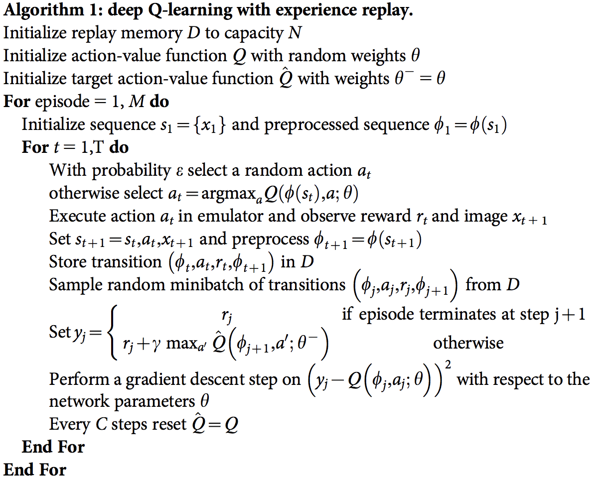
Another two techniques are also essential for training DQN:
- Experience Replay: Since training samples in typical RL setup are highly correlated, and less data-efficient, it will leads to harder convergence for the network. A way to solve the sample distribution problem is adopting experience replay. Essentially, the sample transitions are stored, which will then be randomly selected from the "transition pool" to update the knowledge.
- Separate Target Network: The target Q Network has the same structure as the one that estimates value. Every C steps, according to the above pseudo code, the target network is reset to another one. Therefore, the fluctuation becomes less severe, resulting in more stable trainings.
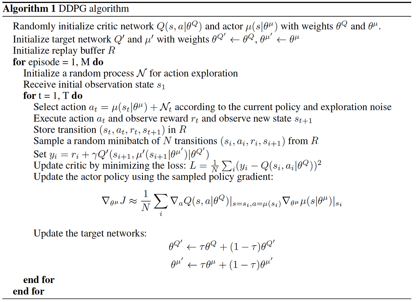
2.4 Deep Deterministic Policy Gradient (DDPG)
Although DQN achieved huge success in higher dimensional problem, such as the Atari game, the action space is still discrete. However, many tasks of interest, especially physical control tasks, the action space is continuous. If you discretize the action space too finely, you wind up having an action space that is too large. For instance, assume the degree of free random system is 10. For each of the degree, you divide the space into 4 parts. You wind up having 4¹⁰ =1048576 actions. It is also extremely hard to converge for such a large action space.
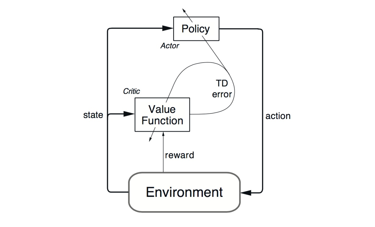
DDPG relies on the actor-critic architecture with two eponymous elements, actor and critic. An actor is used to tune the parameter 𝜽 for the policy function, i.e. decide the best action for a specific state.

A critic is used for evaluating the policy function estimated by the actor according to the temporal difference (TD) error.
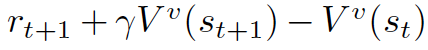
Here, the lower-case v denotes the policy that the actor has decided. Does it look familiar? Yes! It looks just like the Q-learning update equation! TD learning is a way to learn how to predict a value depending on future values of a given state. Q-learning is a specific type of TD learning for learning Q-value.
DDPG also borrows the ideas of experience replay and separate target network from DQN . Another issue for DDPG is that it seldom performs exploration for actions. A solution for this is adding noise on the parameter space or the action space.
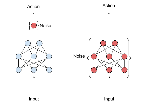
It is claimed that adding on parameter space is better than on action space, according to this article written by OpenAI. One commonly used noise is Ornstein-Uhlenbeck Random Process.
3. Conclusion
I have discussed some basic concepts of Q-learning, SARSA, DQN , and DDPG. In the next article, I will continue to discuss other state-of-the-art Reinforcement Learning algorithms, including NAF, A3C… etc. In the end, I will briefly compare each of the algorithms that I have discussed. Should you have any problem or question regarding to this article, please do not hesitate to leave a comment below or follow me on twitter.
Upmc Td Fascicule Corrige Solution Systeme Procedes Pdf
Source: https://towardsdatascience.com/introduction-to-various-reinforcement-learning-algorithms-i-q-learning-sarsa-dqn-ddpg-72a5e0cb6287